Mixing time of a pseudorandom number generator

Today I was due to speak at the Isaac Newton Institute’s workshop on “Interactions between group theory, number theory, combinatorics and geometry”, which has obviously been canceled. I was going to speak about my work on the Hall–Paige conjecture: see this earlier post. Meanwhile Péter Varjú was going to speak about some other joint work, which I’d like to share with you now.

Consider (if you can consider anything other than coronaviral apocalapyse right now) the random process ${(X_n)}$ in ${\mathbf{Z}/p\mathbf{Z}}$ defined in the following way: ${X_0 = 1}$ (or any initial value), and for ${n\geq 1}$

$\displaystyle X_n = aX_{n-1} + b_n. \ \ \ \ \ (1)$

Here we take ${a}$ to be a fixed integer and ${b_1, b_2, \dots}$ a sequence of independent draws from some finitely supported measure ${\mu}$ on ${\mathbf{Z}}$ . As a representative case, take ${a = 2}$ and ${\mu = u_{\{-1, 0, 1\}}}$ (uniform on ${\{-1, 0, 1\}}$ ).

Question 1 What is the mixing time of ${(X_n \bmod p)}$ in ${\mathbf{Z}/p\mathbf{Z}}$ ? That is, how large must we take ${n}$ before ${X_n}$ is approximately uniformly distributed in ${\mathbf{Z}/p\mathbf{Z}}$ ?

This question was asked by Chung, Diaconis, and Graham (1987), who were motivated by pseudorandom number generation. The best-studied pseudorandom number generators are the linear congruential generators, which repeatedly apply an affine map ${x\mapsto ax+b \bmod p}$ . These go back to Lehmer (1949), whose parameters ${a}$ and ${b}$ were also subject to some randomness (from MathSciNet, “The author’s proposal for generating a sequence of `random’ 8 decimal numbers ${u_n}$ is to start with some number ${u_0\neq 0}$ , multiply it by 23, and subtract the two digit overflow on the left from the two right hand digits to obtain a new number ${u_1}$ .”) The process ${(X_n)}$ defined above is an idealized model: we assume the increment ${b}$ develops under some external perfect randomness, and we are concerned with the resulting randomness of the iterates.

My own interest arises differently. The distribution of ${X_n}$ can be thought of as the image of ${a}$ under the random polynomial

$\displaystyle P_n(X) = X^n + b_1 X^{n-1} + \cdots + b_n,.$

In particular, ${X_n \bmod p = 0}$ if and only if ${a}$ is a root of ${P_n}$ . Thus the distribution of ${X_n \bmod p}$ is closely related to the roots of a random polynomial (of high degree) mod ${p}$ . There are many basic and difficult questions about random polynomials: are they irreducible, what are their Galois groups, etc. But these are questions for another day (I hope!).

Returning to Question 1, in the representative case ${a = 2}$ and ${\mu = u_{\{-1, 0, 1\}}}$ , CDG proved the following results (with a lot of clever Fourier analysis):

The mixing time is at least
$\displaystyle (1+o(1)) \log_2 p.$

This is obvious: ${X_n}$ is supported on a set of size ${O(2^n)}$ , and if ${n \leq (1-\varepsilon) \log_2 p}$ then ${2^n \leq p^{1-\varepsilon}}$ , so at best ${X_n}$ is spread out over a set of size ${p^{1-\varepsilon}}$ .
The mixing time is never worse than
$\displaystyle C \log p \log \log p.$
Occasionally, e.g., if ${p}$ is a Mersenne prime, or more generally if ${a}$ has small order mod ${p}$ (or even roughly small order, suitably defined), the mixing time really is as bad as that.
For almost all odd ${p}$ the mixing time is less than
$\displaystyle 1.02 \log_2 p.$

You would be forgiven for guessing that ${1.02}$ can be replaced with ${1+o(1)}$ with more careful analysis, but you would be wrong! In 2009, Hildebrand proved that for all ${p}$ the mixing time of ${X_n \bmod p}$ is at least

$\displaystyle 1.004 \log_2 p.$

Therefore the mixing time of ${X_n \bmod p}$ is typically slightly more than ${\log_2 p}$ . What is going on here? What is the answer exactly?

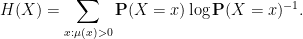
In a word, the answer is entropy. Recall that entropy of a discrete random variable ${X}$ is defined by

$\displaystyle H(X) = \sum_{x : \mu(x) > 0} \mathbf{P}(X = x) \log \mathbf{P}(X = x)^{-1}.$

Here are some basic facts about entropy:

If ${X}$ is uniform on a set of size ${k}$ then ${H(X) = \log k}$ .
Entropy is subadditive: the entropy of the joint variable ${(X, Y)}$ is at most ${H(X) + H(Y)}$ .
Entropy cannot be increased by a (deterministic) function: ${H(f(X)) \leq H(X)}$ .

By combining the second and third facts, we have the additive version (in the sense of adding the variables) of subadditivity:

$\displaystyle H(X + Y) \leq H(X) + H(Y).$

In particular, it follows from (1) that

$\displaystyle H(X_{m+n}) \leq H(X_m) + H(X_n),$

and hence by the subadditive lemma ${H(X_n)/n}$ converges. (We are thinking now of ${X_n}$ as a random variable in ${\mathbf{Z}}$ , not reduced modulo anything.) Call the limit ${H = H(a, \mu)}$ .

It is easy to see in our model case ${a=2, \mu = u_{\{-1, 0, 1\}}}$ that ${H \leq \log 2}$ (because ${X_n}$ has support size ${O(2^n)}$ ). If ${H < \log 2}$ , then it follows that the mixing time of ${X_n \bmod p}$ is strictly greater than ${\log_2 p}$ (as ${X_n}$ cannot approach equidistribution mod ${p}$ before its entropy is at least ${(1+o(1))\log p}$ ).

Indeed it turns out that ${H < \log 2}$ . This is "just a computation": since ${H = \inf_{n\geq 1} H(X_n) / n}$ , we just need to find some ${n}$ such that ${H(X_n) / n < \log 2}$ . Unfortunately, the convergence of ${H(X_n) / n}$ is rather slow, as shown in Figure 1, but we can take advantage of another property of entropy: entropy satisfies not just subadditivity but submodularity

$\displaystyle H(X+Y+Z) + H(X) \leq H(X+Y) + H(X+Z),$

and it follows by a short argument that ${H(X_n) - H(X_{n-1})}$ is monotonically decreasing and hence also convergent to ${H}$ ; moreover, unlike the quotient ${H(X_n)/n}$ , the difference ${H(X_n) - H(X_{n-1})}$ appears to converge exponentially fast. The result is that

$\displaystyle H / \log 2 = 0.98876\dots,$

so the mixing time of ${X_n \bmod p}$ is not less than

$\displaystyle H^{-1} \log p = (1.01136\dots ) \log_2 p.$

(We can also deduce, a posteriori, that we will have ${H(X_n) / n < \log 2}$ for ${n \geq 72}$ , though it is out of the question to directly compute ${H(X_n)}$ for such large ${n}$ .)

Figure 1: The entropy difference rapidly converges. Predicted values are dashed.

This observation was the starting point of a paper that Péter and I have just finished writing. The preprint is available at arxiv:2003.08117. What we prove in general is that the mixing time of ${X_n \bmod p}$ is indeed just ${(H^{-1} + o(1)) \log p}$ for almost all ${p}$ (either almost all composite ${p}$ coprime with ${a}$ , or alternatively almost all prime ${p}$ ). In other words, entropy really is the whole story: as soon as the entropy of ${X_n}$ is large enough, ${X_n \bmod p}$ should be close to equidistributed (with a caveat: see below). The lower bound is more or less clear, as above. Most of the work of the paper is involved with the upper bound, for which we needed several nontrivial tools from probability theory and number theory, as well as a few arguments recycled from the original CDG paper.

However, just as one mystery is solved, another arises. Our argument depends on the large sieve, and it therefore comes with a square-root barrier. The result is that we have to assume ${H(a, \mu) > \frac12 \log a}$ . This is certainly satisfied in our representative case ${a = 2, \mu = u_{\{-1, 0, 1\}}}$ (as the entropy is very close to ${\log 2}$ ), but in general it need not be, and in that case the problem remains open. The following problem is representative.

Problem 2 Let ${a \geq 2}$ and let ${\mu = u_{\{0, 1\}}}$ . Then ${X_n}$ is uniform on a (Cantor) set of size ${2^n}$ , so ${H(a, \mu) = \log 2}$ . Show that the mixing time of ${X_n \bmod p}$ is ${(1+o(1))\log_2 p}$ for almost all primes ${p}$ .

You might call this the “2–3–4–5 problem”. The case ${a=2}$ is trivial, as ${X_n}$ is uniform on ${\{1, \dots, 2^n\}}$ . The case ${a=3}$ is covered by our main theorem, since ${\log 2 > \frac12 \log 3}$ . The case ${a=4}$ is exactly borderline, as ${\log 2 = \frac12 \log 4}$ , and this case is not covered by our main theorem, but we sketch how to stretch the proof to include this case anyway. For ${a \geq 5}$ we need a new idea.